Sponsored Link

Sponsored Link

Wednesday, July 29, 2009

VBA Code to delete worksheets

In my last post we have seen how to add worksheets to Microsoft Excel workbook using VBA code. In this post we will delete the worksheet. Now, you have to be very careful while deleting worksheet because you won’t be able to recover any worksheet that deleted by using this VBA/Macro code. I have written two different set of codes. First one will delete active sheet while other one will delete based on sheet name provided by end user. I have purposely kept the prompt so that you don’t end up loosing any data while testing code.

So, let’s move ahead with first set of VBA/Macro code.

Sub DeleteActiveSheet()

' deletes active worksheet in the active workbook

On Error Resume Next

Dim str As String

str = ActiveSheet.Name

Sheets(str).Delete

End Sub

Warning: The above will permanently delete active worksheet. Kindly be careful.

Mentioned below is a second set of VBA/Macro code.

Sub DeleteSheet()

' deletes a sheet name entered by user in the active workbook

On Error Resume Next

Dim str As String

str = InputBox("Enter the worksheet name", "Findsarfaraz")

Sheets (str).Delete

End Sub

Warning: The above will permanently delete the worksheet name provide by you. Kindly be careful.

I would suggest you to take a look at code in MS Excel file. Click here to download. To view code, press Alt + F11 keys.

If you like to read more such articles, please subscribe to my blog. Click here to subscribe, its free. Also, your comments motivates me. Please comment.

We assure you knowledge, not SPAM!

Read more on this article...

Tuesday, July 28, 2009

VBA code to Add worksheet

Today we will discuss a different method in VBA to add worksheet in MS Excel workbook. Now when I say different method I mean ways of adding worksheet based on your requirement. Let’s moved ahead and start with simple piece of code to complex one in steps and based on scenario.

Scenario 1: Add worksheet with default name.

Sub Addsheet()

Worksheets.Add

End Sub

Note: The above code will add a worksheet before active worksheet.

Scenario 2: Add worksheet with specific name.

Sub Addsheet()

Worksheets.Add().Name = "Sarfaraz"

End Sub

Scenario 3: Add multiple worksheets.

Sub Addsheet3()

'Add Multiple worksheets

Worksheets.Add After:=Worksheets(Worksheets.Count), Count:=4

End Sub

Scenario 4: Add worksheets at end.

Sub Addsheet4()

'Add worksheets at the end

Worksheets.Add(After:=Worksheets(Worksheets.Count)).Name = "Sarfaraz"

End Sub

If you have any issue with replicating this code in MS Excel than download the Microsoft Excel file which I have uploaded. To view the code press Alt + F11 key on keyboard. To run the code I have place four buttons. Each button has one scenario.

Download Add Sheet example

For Free Microsoft Excel and VBA help subscribe to blog via email.

We assure you knowledge, not SPAM!

Read more on this article...
Monday, July 27, 2009

Sequence formula

Many a times you must want MS Excel to sequence the entry automatically. But thats not one of the features of MS Excel. So what you do is you enter the list than you type 1 in the top most row and drag it till last row. isn't it? This is most common practice I have seen around. Today here I will share to tricks on sequence.

In first sequence type, we will count the based on number of rows filled without checking if the value is duplicate with respect to previous row.

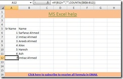
Formula: =IF(B6="","",COUNTA($B$6:B6))

In the above example, we are considering that we are sequencing based on column B starting from 6th row. The formula check if the value is present in B column and then counta find the count of non-blank from column B6 to respective row and returns count. Like, if you are on row 12 then formula will be  =IF(B12="","",COUNTA($B$6:B12)).  Lets take a look at illustration in image below.

Click on image below to view enlarge

Microsoft Excel, Sequence Generator

In second type, the increment happens only if the text entered is different from the one in the previous cell. Like if John is entered in B2 and B3 then both will have sequence number 1. Remember the same number will be assigned only if the both entered text are in adjacent cells like B2 and B3. Also, if you are using this for data entry purpose than to fix the sequence you can sort on the column.

Click on image below to view enlarge

Microsoft Excel, Sequence generator

Formula: =IF(B5="","",IF(B5=B4,A4,A4+1))

First IF checks whether the cells has any value. If the cells is empty then it leaves sequence cell empty(in above example A column has sequence numbers) empty. Else, it checks if the current cells values is same as cell in previous row. if yes, then it returns sequence of previous cell otherwise it adds 1 to sequence of previous row and return new number in sequence. You can concatenate/combine this sequence number with any text to get unique keys like in invoices/bill or memo.

I would suggest you to download the file I have enclosed with post. That will give you more clear picture. Also, I would suggest you to use this trick in one of your MS Excel report or template. So, you can remember entire logic.

Sequence example

Thank you for spending your valuable time in reading above post and if you like to read more such tricks subscribe to blog via email.

We assure you knowledge, not SPAM!

Read more on this article...

Friday, July 24, 2009

Trunc function to remove decimal

This function remove the decimal part of number. I find this function useful only when decimal precision is not important. Like you only want to consider 2 decimal places and want to completely ignore the numbers beyond 2 decimal places or so. The most important thing about Trunc function is it does not round off, it completely removes decimal.

Syntax: Trunc(Number, Precision)

We will take few number for example to explain you how Trunc functions works. Like in all other post, I have enclosed image with example.

Click on image below to view enlarge

Microsoft Excel, trunc

Also, if you face issue with replicating this example on MS Excel than download the MS Excel file with example.  I am sure you will use this function in your day to work life.

Download Example of Trunc

Thank you for spending your valuable time in reading above post and if you like to read more such tricks subscribe to blog via email.

We assure you knowledge, not SPAM!

Read more on this article...

Wednesday, July 22, 2009

Upper function to change case

This post is for beginners of MS Excel. This function convert all the characters to upper case(capitals). It is very useful when you have a data which is not in uniform case.  Like data received from Data entry operators.

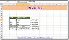
Syntax: =Upper(Text)

Attached below is snapshot with Upper function as example. Take a look, I am sure this will help you.

Click on image below to view enlarge

Microsoft Excel, Upper Function 

There are other function in MS Excel which help you with cases are Lower(), Proper(). Also, the Upper function is very useful when you want to compare text from two cells. Since Exact() function is case sensitive it treats 'a' and 'A' as two different letters. I have enclosed the link to my earlier post where I have demonstrated to find cases using exact function

Check which CASE is used using Exact function

Thank you for spending your valuable time in reading above post and if you like to read more such tricks subscribe to blog via email.

We assure you knowledge, not SPAM!

Read more on this article...
Tuesday, July 21, 2009

Workday function

Workday function is used to find either past or future date before/after the given number of business days. The function only consider working/business days which mean while arriving to date it excludes Weekly off's and holidays. What I like most about this function is you can also provide it with holiday list you don;t want to be considered.

Now if you are thinking what will be the application of this function than let me tell you whenever I decide any dead line for project  I use this function to calculate date. This exclude all Weekends and holidays list which I provide to function. Also, this can be use to calculate delivery date or number of days of work performed.

Let's take a look at the syntax of formula below.

=Workday(StartDate, Days, Holidays)

StartDate is the beginning date

Days are the number of nonweekend and non-holidays days before or after start date which you want to use for calculating end date. Like for example, if you know that delivery of post takes 5 business days than you will input 5 to Days in formula.

Holidays: List of days you want to exclude while calculating end days. Like if you are not working on particular days than you can provide that to formula. This can be provided by using constant arrar {"A", "B","C"} or by range of cells. Remember, Saturday and Sunday are default weekends and will be considered as non working days.

Now lets take look at example of Workday function.

Click on image below view enlarge

workday function, microsoft Excel

To help you in making practical use of this formula I have made an MS Excel file with workday example and one of its application which you can download from link below. I foresee this function to be very useful when for companies who are in courier business. Also, in calculating targets for each employee and understanding time and motion calculation. Please do write to me if you like to discuss this further.

Click here to Download Workday function Example

Kindly do let us know your suggestion about post. Also, you receive free updates, add-ins, ebooks and useful macro code Click Here

We assure you knowledge, not SPAM!

Read more on this article...

Wednesday, July 15, 2009

VBA code, count using color

This is really funny thing in MS Excel I discovered today. Yes, a VBA code to count cells using colors. The intention behind is this post is to share VBA code and help you move ahead with VBA learning. This function is written by me. As you go below you will find formula syntax, vba code and add-ins. So, you can use add-ins on your system without replicating code and you can use this add-in all in open MS Excel file.

Syntax:  =CountColor(TargetRange,CellwithColor)

TargetRange: Range of cells which you wanted to count under which you want to count cells using criteria as another formatted cell.

CellwithColor: Single cell which filled with color which you want to count from TargetRange.

Note: It wont count cells that are formatted conditionally.

It may sound complex, but trust its very simple to use. Take a look at screen shot below where I have illustrated using CountColor.

Microsoft Excel, Count color 

Now, lets take a look a code of function which calculate count based on colors.

Public Function CountColor(target As Range, clr As Range) As Integer

Dim cnt As Integer

cnt = 0

For Each c In target
        If c.Interior.ColorIndex = clr.Interior.ColorIndex Then
            cnt = cnt + 1
        End If
Next c

CountColor = cnt

End Function

Dim cnt as Integer -> declare the integer variable used to count cells.

For each c in Target - > each c refers to one cell in target range while looping through for loop. So, if the target range is A1:A10 then while looping its goes A1, A2, A3.... ,A10.

c.Interior.colorIndex -> Colorindex returns the number for color, Interior of cell refers to color pattern and c is cell from target range. Similarly, clr.Interior.ColorIndex returns the number for color pattern in criteria.  So, if the number returned by getcolorindex method matches with number returned by getcolorindex of criteria it adds 1 to cnt.

After completing the entire range it pass the value to Countcolor.

If you still have doubts, download the count color example file. I am sure you would love to use this function.

Download Count color example

Macro are good to use when you want to process or perform operation in one MS Excel file. However, when you want to use any function/vba code independently in all open MS Excel file than add-ins are the best option. Other good thing about add-ins is they don't prompt whether you want to enable or disable code. Hence, I have uploaded the add-ins for you to use and send it across to your friends. Please feel free to download, its Free.

 Download Countcolor Add-ins

If you need help with installing add-ins, please visit our post How to install Add-ins.

Thanks for spending time in reading post. Request you to leave your comments. Also, you can receive updates, add-ins and e-books, its free.

We assure you knowledge, not SPAM!

Read more on this article...

Tuesday, July 7, 2009

Year Function

Year function is used to extract year from Date. It’s very useful when you want to summarize data at year level or you want to apply filter on year. This function in combination with other function is very useful in calculating past/future dates. I will share few examples of Year function in near future.

Formula: =Year(Date)

Click on image below to view enlarge

Yearfunc

Example1: Find the current year.

Formula: Year(Today())

Click on image below to view enlarge.

yearfuncexam

If you face any issue with replicating this example in MS Excel or understanding this function. I would suggest you to download Year function Excel file enclosed below

Year Function Example

Kindly let me know your view and experiences about using Year function. For free updates subscribe here.

We assure you knowledge, not SPAM!

Read more on this article...

YearFrac Function

Yearfrac functions returns the portion of years between dates. The most recommended format of return is percentage. Like if you take Jan 01, 2009 as start and Jun 30, 2009 as end, YearFrac will return 0.49 which is nothing but 49% of year. 

 Formula: Year(StartDate, EndDate, Basis)

StartDate: StartDate is date as the name suggest is beginning date which you want to be considered for calculation. Like, if you want to calculate fraction of year starting from day one of year than start date will be 01/01/2009.

EndDate: Similar as above will be last date till which you want to find the fraction of year.

Basis: There are five options available for choose based on which you will receive the results. Each Type is mentioned below.

  • 0: US Calendar style where 30 days per month is considered and hence 360 days in a year. Like 30/360. Also, if nothing is provided in basis than by default if consider as 0.
  • 1: This will make formula take actual number of days/actual number of days year consist of.
  • 2: Actual number of days/360.
  • 3: Actual number of days/365.
  • 4: Eurpean 30/360

Basis is a most critical parameter which will be be dependant of type of calendar you follow or you want to use for calculation. So, be sure.

Example 1: We will try to calculate YearFrac using different basis.  Just to keep the example started I will considered fixed dates 7/6/2009 and 8/6/2009 which has different of 31 days between them.

Click on image to view enlarge.

yearfrac

Example 2: Task is to calculate leaves on pro-data basis. Like in a year you can have only 21 leaves. So, as the days passes how many leaves will accumulate.

Click on image to view enlarge.

YearFrac2

Note: in both examples I have formatted Yeafrac as percentage.

If you still have difficulty in using YearFrac function. I would suggest you to download the file with YearFrac Example. Also, I have added on bonus example in this file.

Click Here to download YearFrac

If you are first time visitor I would request you to subscribe our blog via Email. We will send you free tutorials, e-books, Add-ins and macro code.

We assure you knowledge, not SPAM!

Read more on this article...

Monday, July 6, 2009

Format Painter

Format painter is very useful tool when you only wanted to move format of one cell to another or range on worksheet. Using format painter is easiest way to replicate format on the worksheet.

format painter icon  is a format painter icon which you will find on Standard toolbar.

Follow the steps to use format painter to move format.

  1. Select the cell of which you want to copy the format.
  2. Click on the format painter icon icon on Standard toolbar.
  3. The moment you click on Format painter icon, you will see that your cursor has changed to + paintbrush icon.
  4. Now you can apply the format by clicking on single cell or by dragging it on range of cell. However, if you want to apply the format to disjoint/non contiguous cells than steps will be bit different.

Follow the steps to use format painter on non-contiguous cells.

  1. Select the cell of which you want to copy the format.
  2. Double click on the format painter iconformat painter icon on standard toolbar.
  3. Now, like earlier the moment you double click the format painter icon you will see your cursor has change to + paintbrush icon.
  4. Now, click on all the cells of which you want to change the format. Once you are done, press Esc.

During my first few month's as an MIS I used this method to speed up my work. Format painter very well copy the conditional formatting as well which I liked the most. Remember one thing, more you practice, more you learn. So, keep practicing. I have one more idea of moving format which I will share with in future posts. Do miss any post, its Free!.

We assure you knowledge, not SPAM!

Read more on this article...

Wednesday, July 1, 2009

Countif with wildcard criteria

Here we will learn to use wildcard * in Countif function. Task is find count of all cell which starts with A or any character. There may be many ways which I may not be aware of, here I am posting something I tried and it worked. If you are not comfortable with Countif than this post is not for you. I would suggest you to visit my Countif Function.

Syntax for countif function is as follows : Countif(Range, Criteria)

Example: We wanted to find count of names starting with A and Sa from the list of names in A column of sheet. Suppose the names are in A2 to A10 range.

Formula Countif(A1:A10, "A*") will return the count of all names starting with A and Countif(A1:A10, "Sa*")

Click on image to view enlarge.

Microsoft Excel, countif example

Note: Criteria provided in countif is not case sensitive. SA and Sa will be treated as same.

Also, you can use this function with conditional formatting for give specific color to cell starting specific character.

You can also download an Countif with wild card example file. 

Click here to download Countif Example

If you are first time visitor, please subscribe via email to receive updates, add-ins, e-books and lot more.

We assure you knowledge, not SPAM!

Read more on this article...